Six Years to AI: How One Lab Built the Infrastructure That Made AI Useful

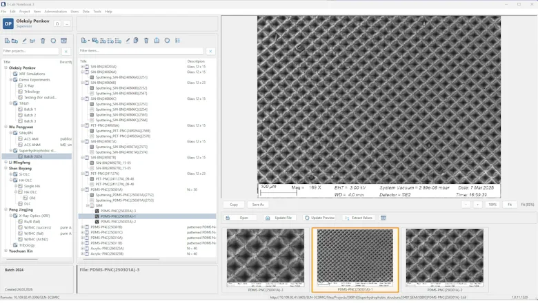
Two scenes

2019, South Korea. A graduate student knocks on the door. The latest Mo/B run came out wrong — the multilayer period drifted. He opens his notebook. The entry reads “Mo/B 300W 120s.” No chamber pressure. No gas flow. No substrate ID. The deposition log? Somewhere on an old computer, in a folder he can’t quite remember. Two hours later we find it: chamber pressure was 50% over spec, almost certainly a flange leak nobody mentioned. Another hour to find the X-ray data — on a USB stick, in a folder called new_new_final. Net result: one lost day, five samples in the bin.

2026, China. I type into a terminal: “Compare deposition logs for samples 260202A and 260202B. Both used identical recipes but different power supplies on the B4C target. Cross-reference with XRR fits.” Thirty seconds later the answer comes back: power supply C delivers 6% more power than B at the same current setpoint, which explains the systematically thicker WC interfaces in the C-deposited samples. Four file formats. Eight data files. Minutes instead of days.

The question is the same one I’ve been asking for fifteen years, first in Korea and now in China: this coating came out wrong, why? What’s different in the second scene isn’t the AI. It’s that for the first time, the data needed to answer the question was actually there to be read.

The data problem nobody writes papers about

Every experimental physics lab generates a lot of data: diffractograms, micrographs, deposition logs, mechanical test results, process parameters. Most labs manage that data poorly — each in their own particular way.

Some people keep paper notebooks. Entries are terse — “Mo/B 300W good.” A week later nobody remembers what “good” meant. The student defends, leaves, takes the context with them.

Others build elaborate folder trees: 2022/March/Week2/Mo-B/attempt3_final_FINAL2/. Two hundred gigabytes of meticulously sorted files that only the author can navigate, and only for about six months.

A third type lives in Excel — one master file, forty-seven tabs, formulas referencing a “Raw Data (old)” sheet that points to an external file on a different computer. It opens in three minutes. On someone else’s machine, not at all.

I’ve been each of these at different points. The failures aren’t a moral problem; they’re a structural one. Nothing in graduate training teaches you how to organize data so that it survives the next student. You invent something, it works for you, and a year after you leave nobody can read it.

None of these approaches solves the actual problem: connecting the process to the result. You ran fifty Mo/B depositions last year. Which deposition parameters correlate with the highest reflectivity? Answering that question requires manually pairing deposition logs with diffraction data for every sample — and discovering that three logs are missing, two diffractograms are unlabeled, and one sample is named differently in the notebook than on the disk.

That isn’t research. That’s archaeology.

The unsexy years

Digitalization didn’t start with a grand plan. It started in 2020 with magnetron sputter deposition control software that ran the carousel, the power supplies, the shutters, the ion gun — because the alternative was standing next to the chamber for five hours per sample.

The deposition control was the visible deliverable. The interesting side effect was a 32-channel TSV log: chamber pressure, voltage, current, power, gas flows, shutter states, carousel position — every parameter, every second. About 1.5 MB of plain text per run. We didn’t think much about the logs at the time — they were a debugging tool, nothing more. Six years later they turned out to be the most valuable artifact the software produced.

In January 2021 the electronic lab notebook went live. The hierarchy mirrors how lab work actually flows:

Project → Folder → Specimen → Action → Files

Every physical sample is a Specimen with a name, substrate type, and an Outcome field for the headline result. Every operation on it — deposition, annealing, XRD, SEM, indentation, scratch test — is an Action attached to specific equipment. Raw data files live with the action that produced them: .xrdml from the diffractometer, .xrcx from X-Ray Calc (our open-source XRR fitter), .dsc recipe files, .mit indentation results. Beyond files, each action carries structured key-values — multilayer period, hardness, friction coefficient, roughness — the numbers you actually want to query across hundreds of samples.

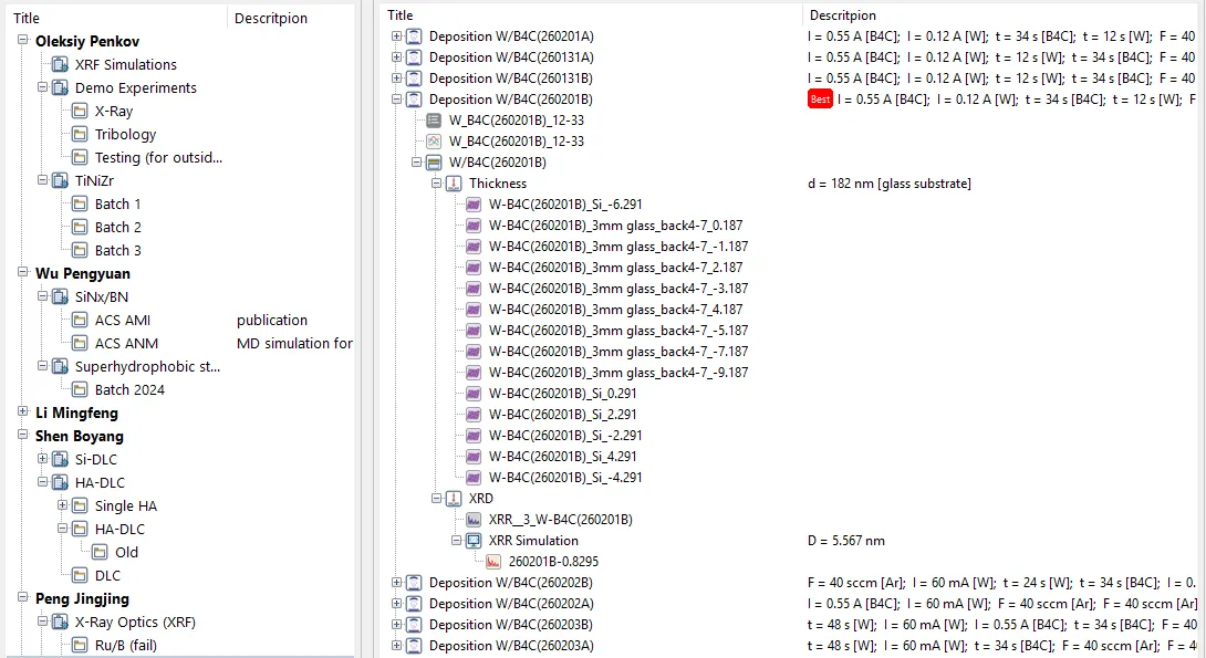
The hierarchy: project → folder → specimen → action → files. Every measurement lives where you’d expect to find it.

What followed was years of unglamorous discipline. Every sample registered. Every diffractogram uploaded and tagged. Every deposition log filed against the right action. Every key-value entered. Plugins to extract structured data from each instrument’s proprietary format, so the numbers became queryable instead of locked inside vendor software.

Was it boring? Mind-numbingly. The discipline came close to breaking down half a dozen times — usually right after a paper deadline, when the temptation to skip the entry and “come back to it later” was strongest. The trick wasn’t willpower. The trick was making the system fast enough that recording the data was less work than skipping it: keyboard shortcuts, smart defaults, plugins that pre-filled half the entry from the file you’d just dropped in.

That’s the part of digitalization nobody publishes papers about. By 2026: 19 projects, hundreds of specimens, thousands of files. A continuous five-year history.

The detective story

In March 2026 we ran a series of W/B4C multilayer mirrors — 30 bilayers, for X-ray fluorescence optics. Two pulsed DC supplies in the chamber, labeled B and C. We rotated which physical supply drove which target across the series, expecting the choice to be irrelevant. Identical recipes. Identical setpoints. Identical everything except the supply.

The XRR fits disagreed.

My first guess was that something subtle had drifted between the runs — but identical recipes meant the variables I knew about were already controlled. So I asked Claude — connected to the lab notebook through a Model Context Protocol server we’d written — to figure out what I’d missed.

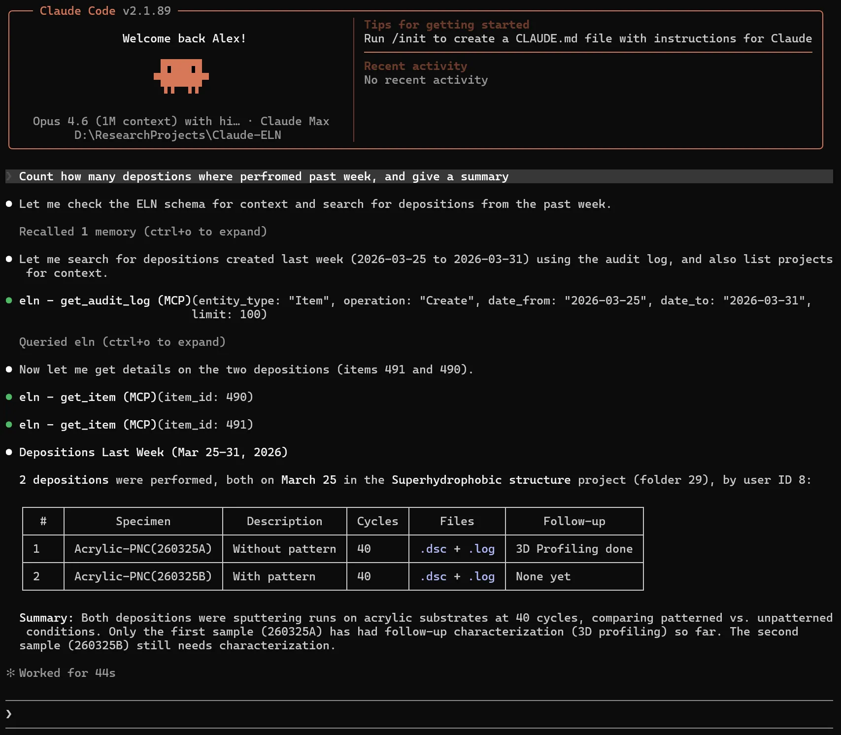
Claude calling MCP tools — get_experiment, extract_file_data, correlate_values — to walk the database the same way a researcher would.

Step one: the AI pulled the recipe files (.dsc) for both series and compared them byte-by-byte. They were identical except for the line specifying which supply drove the target.

Step two: it parsed the 32-channel deposition logs. Same 550 mA setpoint on both supplies — but supply C was actually delivering 464–478 V where supply B sat at 458–471 V. About 6% more power, undocumented anywhere except in the logs.

Step three: it pulled the XRR-fit files (.xrcx) and read out the layer-by-layer thicknesses. Samples deposited with supply C had a WC interface of 20.4 nm at 48 s of W deposition. Samples with supply B: 9.1 nm under the same nominal conditions.

Step four: it wrote up the conclusion. Higher delivered power on supply C means higher ion energy at the W/B4C interface, which drives more interlayer mixing. Recommendation: cross-calibrate the supplies before running any further comparative experiments.

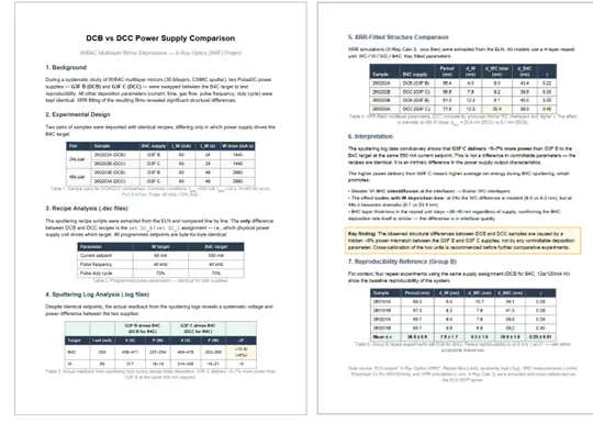
Final report, generated end-to-end from the natural-language question. Tables, conclusions, and a recommendation — ready to paste into a lab meeting.

Four file formats. Eight data files. Four experiments plus four controls. A scientist could have done the same investigation — in a day or two of careful work. The AI did it in minutes.

But only because the data was already there. Structured. Linked to specimens. Reachable through an API. If the logs had been “somewhere on the old computer” and the diffractograms on a USB stick in new_new_final, no AI in the world would have helped.

What it actually took

Everyone is excited about AI in science right now. Conference talks on AI-driven materials discovery. Papers on machine learning for thin-film optimization. Mandatory AI mentions in every grant proposal.

Almost all of that work starts with the same quiet assumption: we have a clean, structured dataset. Where the dataset comes from is rarely the topic.

The truth is that most labs don’t have the digital foundation to use AI on their own data at all. Their data lives in notebooks, Excel files, USB sticks, and the heads of recently graduated students. Language models can’t read handwriting and they can’t recover what was never recorded.

Our integration timeline tells the story plainly enough. Connecting Claude to the notebook took a day. Writing the MCP server took two weeks. Building the infrastructure underneath it took six years — and that’s the part you can’t compress.

The deposition control software. The lab notebook. The data extractors. And — far more important than any of those — the daily habit of registering every sample, uploading every measurement, filling in every parameter. Without that habit, AI is just a chatbot that can confidently discuss thin-film physics while having no idea your power supply has been drifting for three weeks.

The first run is always the hardest. Mo(210121-A) — molybdenum on a 10×10 mm silicon substrate, January 2021 — was the first specimen we ever entered. Nothing about the entry was inherently valuable. What was valuable was that everything after it followed the same rules.